<?xml version="1.0" encoding="utf-8"?><feed xmlns="http://www.w3.org/2005/Atom" ><generator uri="https://jekyllrb.com/" version="3.10.0">Jekyll</generator><link href="https://spencer.wtf/feed.xml" rel="self" type="application/atom+xml" /><link href="https://spencer.wtf/" rel="alternate" type="text/html" /><updated>2026-02-20T11:10:56+00:00</updated><id>https://spencer.wtf/feed.xml</id><title type="html">spencer.wtf</title><subtitle>Spencer Dixon is a Senior Ruby and Python Developer with 11+ years of experience building software for UK Government Digital Services and global conservation efforts. Technical articles on ruby, python and software architecture.</subtitle><author><name>Spencer Dixon</name></author><entry><title type="html">Cleaning up merged git branches: a one-liner from the CIA’s leaked dev docs</title><link href="https://spencer.wtf/2026/02/20/cleaning-up-merged-git-branches-a-one-liner-from-the-cias-leaked-dev-docs.html" rel="alternate" type="text/html" title="Cleaning up merged git branches: a one-liner from the CIA’s leaked dev docs" /><published>2026-02-20T00:00:00+00:00</published><updated>2026-02-20T00:00:00+00:00</updated><id>https://spencer.wtf/2026/02/20/cleaning-up-merged-git-branches-a-one-liner-from-the-cias-leaked-dev-docs</id><content type="html" xml:base="https://spencer.wtf/2026/02/20/cleaning-up-merged-git-branches-a-one-liner-from-the-cias-leaked-dev-docs.html"><![CDATA[<p>In 2017, WikiLeaks published Vault7 - a large cache of CIA hacking tools and internal documents. Buried among the exploits and surveillance tools was something far more mundane: <a href="https://wikileaks.org/ciav7p1/cms/page_1179773.html">a page of internal developer documentation with git tips and tricks</a>.</p>

<p>Most of it is fairly standard stuff, amending commits, stashing changes, using bisect. But one tip has lived in my <code>~/.zshrc</code> ever since.</p>

<h2 id="the-problem">The Problem</h2>

<p>Over time, a local git repo accumulates stale branches. Every feature branch, hotfix, and experiment you’ve ever merged sits there doing nothing. <code>git branch</code> starts to look like a graveyard.</p>

<p>You can list merged branches with:</p>

<pre><code class="language-bash">git branch --merged
</code></pre>

<p>But deleting them one by one is tedious. The CIA’s dev team has a cleaner solution:</p>

<h2 id="the-original-command">The original command</h2>

<pre><code class="language-bash">git branch --merged | grep -v "\*\|master" | xargs -n 1 git branch -d
</code></pre>

<p>How it works:</p>

<ul>
  <li><code>git branch --merged</code> — lists all local branches that have already been merged into the current branch</li>
  <li><code>grep -v "\*\|master"</code> — filters out the current branch (<code>*</code>) and <code>master</code> so you don’t delete either</li>
  <li><code>xargs -n 1 git branch -d</code> — deletes each remaining branch one at a time, safely (lowercase <code>-d</code> won’t touch unmerged branches)</li>
</ul>

<h2 id="the-updated-command">The updated command</h2>

<p>Since most projects now use <code>main</code> instead of <code>master</code>, you can update the command and exclude any other branches you frequently use:</p>

<pre><code class="language-bash">git branch --merged origin/main | grep -vE "^\s*(\*|main|develop)" | xargs -n 1 git branch -d
</code></pre>

<p>Run this from <code>main</code> after a deployment and your branch list goes from 40 entries back down to a handful.</p>

<p>I keep this as a git alias so I don’t have to remember the syntax:</p>

<pre><code class="language-bash">alias ciaclean='git branch --merged origin/main | grep -vE "^\s*(\*|main|develop)" | xargs -n 1 git branch -d'
</code></pre>

<p>Then in your repo just run:</p>

<pre><code class="language-bash">ciaclean
</code></pre>

<p>Small thing, but one of those commands that quietly saves a few minutes every week and keeps me organised.</p>]]></content><author><name>Spencer Dixon</name></author><category term="git" /><category term="productivity" /><category term="tools" /><summary type="html"><![CDATA[How to delete all merged git branches locally with a single command. This one-liner has been in my zshrc since 2017 — I found it buried in the CIA's Vault7 leaked developer docs.]]></summary></entry><entry><title type="html">Progressive Web Apps with Rails</title><link href="https://spencer.wtf/2024/06/10/progressive-web-apps-with-rails.html" rel="alternate" type="text/html" title="Progressive Web Apps with Rails" /><published>2024-06-10T09:54:00+00:00</published><updated>2024-06-10T09:54:00+00:00</updated><id>https://spencer.wtf/2024/06/10/progressive-web-apps-with-rails</id><content type="html" xml:base="https://spencer.wtf/2024/06/10/progressive-web-apps-with-rails.html"><![CDATA[<p>Rails 8 will ship with the files necessary to make your application a Progressive Web App (PWA) by default.</p>

<p>As a Rails developer, I’m a big fan of PWAs. The idea of offering a “good enough” mobile app experience from the same codebase is a huge advantage for small teams and solo developers who don’t have the luxury of the time or money needed to maintain a dedicated mobile app codebase.</p>

<p>The good news is that converting your app to a PWA isn’t hard. You can do it in about 10-15 minutes. Adding native notifications and offline mode might take you a bit longer, but getting your app to be downloadable to a home screen and function like a mobile app is fairly straightforward.</p>

<p>We can take a look at the <a href="https://github.com/rails/rails/pull/50528/files">PR</a> for PWA default files in Rails 8 and take inspiration from this to make our Rails &lt;8 apps PWA ready.</p>

<h2 id="1-add-the-metatags-to-your-layout">1. Add the metatags to your layout</h2>

<pre><code class="language-html">&lt;head&gt;
  &lt;meta name="apple-mobile-web-app-capable" content="yes"&gt;
  &lt;link rel="manifest" href="/manifest.json"&gt;
&lt;/head&gt;
</code></pre>

<p>The MVP for a PWA is to serve a <code>manifest.json</code> at the root path of your project. This file contains the config for your PWA, details like the name that should be used for the app, the app icon, a description etc.</p>

<h2 id="2-add-a-pwa-controller-to-serve-the-manifestjson">2. Add a PWA controller to serve the manifest.json</h2>

<pre><code class="language-ruby">class PwaController &lt; ApplicationController
  protect_from_forgery except: :service_worker

  def service_worker
  end

  def manifest
  end
end
</code></pre>

<p><code>service_worker.js</code> can be thought of as our bridge between our PWA mobile app and our web app. It’s capable of doing things like intercepting requests and it’s where we’d do things like offline mode should we wish to. It isn’t strictly needed for transforming our Rails app into a very basic PWA, but we’ll deliver an empty file for now so it’s there to expand on later.</p>

<h2 id="3-hook-up-the-routes-for-the-pwa-controller">3. Hook up the routes for the PWA controller</h2>

<p>In our <code>config/routes.rb</code></p>

<pre><code class="language-ruby">get "/service-worker.js" =&gt; "pwa#service_worker"
get "/manifest.json" =&gt; "pwa#manifest"
</code></pre>

<h2 id="4-serve-our-default-pwa-files">4. Serve our default PWA files</h2>

<p>Create a new directory at <code>app/views/pwa</code></p>

<p>We’ll add an empty <code>service_worker.js</code> here, and then add another file called <code>manifest.json.erb</code>.</p>

<p>Copy in the following. Note that since we used the <code>.json.erb</code> extension, we can use the <code>image_path</code> helper here to pull a 192x192 and 512x512 icon image into the json file. These two image sizes are the bare minimum you need to serve a PWA so make sure your images conform to these sizes and that you have both in the root of your <code>assets/images</code> directory.</p>

<p>I’ve found <a href="https://realfavicongenerator.net/">this site</a> helpful for creating these app icons. You can upload a high res icon and get back a zip file of icons in the right sizes and formats.</p>

<pre><code class="language-json">{
  "short_name": "Soju",
  "name": "Soju",
  "id": "/",
  "icons": [
    {
      "src": "&lt;%= image_path 'android-chrome-192x192.png' %&gt;",
      "sizes": "192x192",
      "type": "image/png"
    },
    {
      "src": "&lt;%= image_path 'android-chrome-512x512.png' %&gt;",
      "sizes": "512x512",
      "type": "image/png"
    }
  ],
  "start_url": "/",
  "background_color": "#fafafa",
  "display": "standalone",
  "scope": "/",
  "theme_color": "#fafafa"
}
</code></pre>

<p>That’s all there is to making your app a very basic PWA!</p>

<p>Commit and host it and you should be able to “Add to Home Screen” when viewing the website in Safari on iOS. The app will save to your home screen, functioning just the same as a mobile app.</p>

<p>It’s a great solution for providing the mobile experience without the overhead of maintaining a dedicated mobile codebase.</p>]]></content><author><name>Spencer Dixon</name></author><category term="rails" /><category term="pwa" /><category term="mobile" /><summary type="html"><![CDATA[Learn how to convert your Rails application into a Progressive Web App (PWA) in 10-15 minutes. Covers manifest.json, service workers, and upcoming Rails 8 PWA defaults.]]></summary></entry><entry><title type="html">Granular Polymorphic User Permissions with Cancancan</title><link href="https://spencer.wtf/2022/03/29/granular-polymorphic-user-permissions-with-cancancan.html" rel="alternate" type="text/html" title="Granular Polymorphic User Permissions with Cancancan" /><published>2022-03-29T16:08:00+00:00</published><updated>2022-03-29T16:08:00+00:00</updated><id>https://spencer.wtf/2022/03/29/granular-polymorphic-user-permissions-with-cancancan</id><content type="html" xml:base="https://spencer.wtf/2022/03/29/granular-polymorphic-user-permissions-with-cancancan.html"><![CDATA[<p>I’ve recently been refactoring how user permissions work in a project to be more granular.</p>

<p>In this project, users are members of organisations, and organisations have many funds and needs.</p>

<p>The manager of the organisation can CRUD these funds and needs, but a regular user should only be able to read them, unless given special permission. This special permission would work on a per-item basis.</p>

<p>Users should also be able to read or manage funds from outside of their organisation if they have been granted special access, by someone within the organisation.</p>

<p>This sounds complex, but the tl;dr is this:</p>

<ul>
  <li>Members of an organisation can see things inside that organisation</li>
  <li>Managers of the organisation can CRUD things in that organisation</li>
  <li>Granting a special permission between a user and a specific item supersedes any organisation permissions and means that user can access that thing according to whichever read/write role specified in the special permission.</li>
</ul>

<p>At it’s core, we want to be able to store a record in the database that say “this user has this type of permission to access this item”.</p>

<p>Once we’re storing this in the database, we can use Cancancan to write policies on who should be able to CRUD what, depending on their stored permissions.</p>

<h2 id="implementation">Implementation</h2>

<p>First, we’ll create a table to store our user permissions in our database. These records will link a user, with a given accessible item (either a Fund, Need or Organisation), and we’ll also have a column for what type of access they’ll have; read or write.</p>

<pre><code class="language-ruby">class CreatePermissions &lt; ActiveRecord::Migration[7.0]
  def change
    create_enum :permission_role, ["read", "write"]

    create_table :permissions, id: :uuid do |t|
      t.references :user, null: false, foreign_key: true, type: :uuid
      t.references :accessible, polymorphic: true, null: false, type: :uuid
      t.enum :role, enum_type: :permission_role, default: "read", null: false

      t.timestamps
    end
  end
end
</code></pre>

<p>We’ll then fill out our model for our new Permissions table</p>

<pre><code class="language-ruby">class Permission &lt; ApplicationRecord
  belongs_to :user
  belongs_to :accessible, polymorphic: true

  enum role: {
    read: "read",
    write: "write"
  }, suffix: true
end
</code></pre>

<p>I like to use <code>suffix: true</code>, which means rails will generate some helper methods for getting and setting roles made by joining our role and enum names, for example: <code>permission.read_role?</code></p>

<p>Now we can add the other side of our permissions association to our user model, as well as each model we want to make “accessible”.</p>

<pre><code class="language-ruby">class User &lt; ApplicationRecord
  has_many :organisations, through: :permissions, source: :accessible, source_type: "Organisation"
	has_many :permissions, dependent: :destroy
end
</code></pre>

<pre><code class="language-ruby">class Organisation &lt; ApplicationRecord
	has_many :funds
	has_many :needs
	has_many :users, through: :permissions
	has_many :permissions, as: :accessible, dependent: :destroy
end
</code></pre>

<pre><code class="language-ruby">class Fund &lt; ApplicationRecord
	belongs_to :organisation
	has_many :permissions, as: :accessible, dependent: :destroy
end
</code></pre>

<pre><code class="language-ruby">class Need &lt; ApplicationRecord
	belongs_to :organisation
	has_many :permissions, as: :accessible, dependent: :destroy
end
</code></pre>

<p>Now we’re set up. You should be able to create a permission record in the console…</p>

<pre><code class="language-ruby">user = User.first
fund = Fund.first

Permission.create(user: user, accessible: fund)
</code></pre>

<p>Next we want to define the rules around who can access what. I’m using Cancancan for permissions, which generates an <code>app/models/ability.rb</code> file to store our access rules.</p>

<pre><code class="language-ruby"># frozen_string_literal: true

class Ability
  include CanCan::Ability

  def initialize(user)
    if user.admin?
      can :manage, :all
    else
      can :manage, [Fund, Need] do |accessible|
        # Can manage an accessible item via write permission for the organisation it belongs to
        Permission.find_by(accessible: accessible.organisation, user: user, role: "write")
      end

      can :read, [Fund, Need] do |accessible|
        # Can read an accessible item via write permission for the organisation it belongs to
        Permission.find_by(accessible: accessible.organisation, user: user, role: "read")
      end

      # Can read/manage an item if I have direct permission (overrides org level permissions)
      can :manage, [Fund, Need, Organisation], permissions: { user: user, role: "write" }
      can :read, [Fund, Need, Organisation], permissions: { user: user, role: "read" }
    end
  end
end
</code></pre>

<p>At the very top level, I let admin level users manage everything (this is just a boolean <code>admin?</code> column on the user model).</p>

<p>If a user is not an admin, the first thing I want to check is if they are a member of the organisation for the accessible item they’re trying to do something with.</p>

<p>I have two rules here, one for read level access, and once for write.</p>

<p>Every accessible item that isn’t an organisation can go here as long as they belong to an organisation and we can call <code>.organisation</code> on them.</p>

<p>Lastly, we have a read and a write rule for checking direct permissions (a link between a user and an accessible item directly without checking through the organisation), we can add organisations here too since a user can have a direct association with an organisation.</p>

<p>Putting access rules in this order means that if we have an accessible item, we check to see if we are a member of its organisation first.</p>

<p>If not, we check to see if we have a direct special permission with that item, and supersede the organisation level permissions.</p>

<p>I think this is a really elegant solution to complex permissions. It’s a lot of flexibility with surprisingly little code.</p>

<p>You can also add tests in your <code>spec/models/user_spec.rb</code> like this. This covers the various combinations of who can access what, and leaves a documentation trail for other developers.</p>

<pre><code class="language-ruby">require "rails_helper"
require "cancan/matchers"

RSpec.describe User, type: :model do
	describe "abilities" do
    subject(:ability) { Ability.new(user) }

    context "when an admin user" do
      let(:user) { create(:user, admin: true) }

      it { is_expected.to be_able_to(:manage, :all) }
    end

    context "when a manager of an organisation" do
      let(:user) { create(:user, admin: false) }
      let(:organisation) { create(:organisation) }
      let!(:external_organisation) { create(:organisation) }
      let!(:permission) { create(:permission, user: user, accessible: organisation, role: "write") }

      let!(:organisation_fund) { create(:fund, organisation: organisation) }
      let!(:organisation_need) { create(:need, organisation: organisation) }
      let!(:external_fund) { create(:fund, organisation: external_organisation) }
      let!(:external_need) { create(:need, organisation: external_organisation) }

      it { is_expected.to be_able_to(:manage, organisation_fund) }
      it { is_expected.to be_able_to(:manage, organisation_need) }
      it { is_expected.not_to be_able_to(:read, external_fund) }
      it { is_expected.not_to be_able_to(:read, external_need) }

      context "with read permission for an external fund" do
        let!(:permission) { create(:permission, user: user, accessible: external_fund, role: "read") }

        it { is_expected.to be_able_to(:read, external_fund) }
        it { is_expected.not_to be_able_to(:manage, external_fund) }
      end
      context "with write permission for an external fund" do
        let!(:permission) { create(:permission, user: user, accessible: external_fund, role: "write") }

        it { is_expected.to be_able_to(:manage, external_fund) }
      end
    end

    context "without being a member of an organisation" do
      let(:user) { create(:user, admin: false) }
      let(:organisation) { create(:organisation) }
      let!(:fund) { create(:fund, organisation: organisation) }
      let!(:need) { create(:need, organisation: organisation) }

      context "when reading a fund belonging to the organisation" do
        it { is_expected.not_to be_able_to(:read, fund) }
      end

      context "when reading a fund belonging to the organisation" do
        it { is_expected.not_to be_able_to(:read, need) }
      end

      context "with a read permission record" do
        let!(:fund_permission) { create(:permission, user: user, accessible: fund, role: "read") }
        let!(:need_permission) { create(:permission, user: user, accessible: need, role: "read") }

        it { is_expected.to be_able_to(:read, fund) }
        it { is_expected.to be_able_to(:read, need) }
      end

      context "with a write permission record" do
        let!(:fund_permission) { create(:permission, user: user, accessible: fund, role: "write") }
        let!(:need_permission) { create(:permission, user: user, accessible: need, role: "write") }

        it { is_expected.to be_able_to(:manage, fund) }
        it { is_expected.to be_able_to(:manage, need) }
      end
    end
	end
end
</code></pre>

<p>Lastly, I’m using GraphQL for the API in this application, so to restrict a query, we can use the <code>.can?</code> method on our ability class with the current user, fund, and permission we want to check for to return a boolean and a surrounding if statement to decide if we return the query or raise an error.</p>

<pre><code class="language-ruby">module Queries
  class Fund &lt; Queries::BaseQuery
    description "Find a specific fund"

    argument :id, ID, required: true

    type Types::FundType, null: false

    def ready?(**args)
      authenticate
    end

    def resolve(id:)
      fund = ::Fund.find(id)

      if Ability.new(current_user).can?(:read, fund)
        fund
      else
        unauthorized_error
      end
    rescue ActiveRecord::RecordNotFound =&gt; error
      raise GraphQL::ExecutionError.new(error)
    end
  end
end
</code></pre>]]></content><author><name>Spencer Dixon</name></author><category term="rails" /><category term="cancancan" /><category term="permissions" /><category term="authorization" /><summary type="html"><![CDATA[Implement fine-grained polymorphic user permissions in Rails using Cancancan. Handle organization-level and item-specific access control with special permission grants.]]></summary></entry><entry><title type="html">De-spaghettifying Rails Apps with Wisper</title><link href="https://spencer.wtf/2022/03/16/despaghettifying-rails-apps-with-wisper.html" rel="alternate" type="text/html" title="De-spaghettifying Rails Apps with Wisper" /><published>2022-03-16T17:21:00+00:00</published><updated>2022-03-16T17:21:00+00:00</updated><id>https://spencer.wtf/2022/03/16/despaghettifying-rails-apps-with-wisper</id><content type="html" xml:base="https://spencer.wtf/2022/03/16/despaghettifying-rails-apps-with-wisper.html"><![CDATA[<p>Let’s say we have a Rails application that users can sign up to, and we want to add a feature to send new users a welcome email on registration. Where should we put that logic?</p>

<h2 id="option-1-the-controller">Option 1: The controller</h2>

<p>We could put it inside our call to create the user in the user registration controller.</p>

<p>Something like this…</p>

<pre><code class="language-ruby">class Registrations
	def create
		user = User.new(user_params)

		if user.save?
			# Send the welcome email if a user is saved successfully
			UserMailer.with(user: resource).welcome_email.deliver_later
			redirect_to root_path, notice: "Signed up!"
		else
			redirect_to root_path, notice: "Could not create account"
		end
	end
end
</code></pre>

<p>I’d argue that putting this logic in the controller is fine for small things, but it’s not the best solution.</p>

<p>If our app starts to grow and we need to do more things like store a “sign up event” to our database, or send a notification to slack to say we’ve acquired a new user, then our controller starts to bloat pretty quickly with a lot of non-registration related logic.</p>

<h2 id="option-2-callbacks">Option #2: Callbacks</h2>

<p>We could use an <code>after_create</code> callback in our User model, but I like this even less. Creating users in the console for test purposes would fire off an unwanted welcome email, and we’re coupling mailer code tightly to our model.</p>

<p>Shoehorning these things into the controller feels messy, and they don’t feel at home in our models either.</p>

<p>So what’s the solution?</p>

<h2 id="option-3-pubsub-style-events-with-wisper">Option #3: Pub/Sub style events with Wisper</h2>

<p>Wisper is a minimalist ruby library that allows us to broadcast events, and listen for them somewhere else in our codebase.</p>

<p>Wisper gives us a simple pattern for dealing with this problem by decoupling code and just passing messages around instead.</p>

<p>Whenever something happens that we want to care about, like the creation of a new user, we’ll send out a <code>:user_created</code> event and have a listener somewhere else that picks up these events, and sends the mailer.</p>

<h2 id="installation">Installation</h2>

<p>Let’s start by installing wisper in our gemfile…</p>

<pre><code class="language-ruby">gem 'wisper'
</code></pre>

<h2 id="events">Events</h2>

<p>Wisper usually passes around raw data, but I prefer to create classes for specific events. Let’s create an event for our user creation. I tend to put these in <code>app/lib/events</code> or <code>app/models/events</code>.</p>

<pre><code class="language-ruby">class Events::UserCreated
	attr_reader :user

	def initializer(user:)
		@user = user
	end
end
</code></pre>

<h2 id="broadcasting-an-event">Broadcasting an Event</h2>

<p>To broadcast an event, we need to include <code>Wisper::Publisher</code> in the code we want to broadcast from. We’re broadcasting from the model, but we can use the same include to broadcast from a controller or anywhere else.</p>

<pre><code class="language-ruby">class User &lt; ApplicationRecord
	include Wisper::Publisher

	has_one :address

	after_create :broadcast_user_created_event

	private

	def broadcast_user_created_event
		broadcast(:user_created, Events::UserCreated.new(user: self))
	end
end
</code></pre>

<p>Wisper’s <code>broadcast</code> method takes two arguments, the first is the event name as a symbol, the second is the payload. This could be a hash, string or any bit of data, but this is where using classes for events really pays off.</p>

<h2 id="listening-and-responding-to-events">Listening and Responding to Events</h2>

<p>Once we’ve got our events, we’ll need to create a Listener to respond to them. I like to put listeners in <code>app/lib/listeners</code> (more about naming conventions later)</p>

<pre><code class="language-ruby">class Listeners::UserListener
  def on_user_created(event)
		UserMailer.with(user: event.user).welcome_email.deliver_late
  end
end
</code></pre>

<p>Our listener should define methods with the same name as the event name. In this case, our event is called <code>:user_created</code>, so we should define a method called <code>on_user_created</code> that accept a single argument; the event payload we passed in to our <code>broadcast</code> method.</p>

<p>“Wait where does <code>on_</code> come from?”</p>

<p>Good question. It’s a stylistic choice, you don’t have to have the prefix, but I prefer it. It happens when you subscribe your listener, which we’ll cover next…</p>

<h2 id="subscribe-your-listener-to-events">Subscribe your Listener to Events</h2>

<p>Our Listener doesn’t automatically pick up events unfortunately, we need to subscribe our listener. We’ll do this in an initializer file…</p>

<pre><code class="language-ruby">Rails.application.config.to_prepare do
  # Wisper subscribers need to be refreshed here when we are in
  # dev/test. This is due to code-reloading, which could re-subscribe
  # existing handlers, leading to duplicates and errors
  Wisper.clear if Rails.env.development? || Rails.env.test?

  # Subscribe your listeners here, use prefix: :on to get event names like on_fund_created in the listener
  Wisper.subscribe(Listeners::FundListener.new, prefix: :on)
end
</code></pre>

<p>Here we’re setting the <code>prefix: :on</code> option, which changes the incoming method in our listener from <code>user_created</code> to <code>on_user_created</code>. This is a matter of preference, but I think it reads nicer with prefixes enabled.</p>

<h2 id="done">Done!</h2>

<p>Your new events bus is now wired up and ready to go! Creating a user should now emit an event that gets picked up by your listener and fires off a welcome email.</p>

<p>It’s a little setup, but the reward for decoupling this code pays off, especially when you start dealing with a few different events.</p>

<h2 id="some-useful-conventions">Some useful conventions</h2>

<p>Here’s some conventions I’ve found useful to help to keep events stuff organised. I tend to document these in the project README too for other developers to follow.</p>

<p>I like to use classes with keyword arguments for events to give them a defined and documented structure. You can also use Structs or Dry Struct to further enforce events to have required attributes and formats.</p>

<p>I create two folders to house all my wisper stuff; <code>app/lib/events/</code> to house my event classes, and <code>app/lib/listeners/</code> to house the corresponding listeners. (Although you could move events to <code>models/events/</code> if you needed to persist some to the database)</p>

<p>I name events <code>Events::ThingVerb</code>, where <code>Thing</code> is usually the model name, and <code>Verb</code> is the past tense action that’s happening to it (created, updated, committed, etc), but feel free to adopt a convention that makes sense for your app, and then document it in your README.</p>

<p>This is what my file structure looks like:</p>

<pre><code class="language-ruby">/app
	/lib
		/events
			user_created.rb
			user_updated.rb
		/listeners
			user_listener.rb
		/publishers
			events_publisher.rb
</code></pre>

<p>When subscribing a listener, I prefer using the <code>prefix: :on</code> option, so that events arrive at my listener with the naming convention <code>on_user_created</code>. I think it reads a bit better than the raw event name.</p>

<p>When using callbacks like <code>after_save</code>, I like to hand these off to a method with the convention <code>broadcast_event_name_event</code>, for example: <code>broadcast_user_created_event</code>. This helps create a consistent naming between my events, listeners, and anything calling them.</p>

<h2 id="publishers-for-easier-calling">Publishers for easier calling</h2>

<p>“But passing in the event name as a symbol and the event object to <code>broadcast</code> feels like duplicating effort, can’t we just pass the event on its own?”</p>

<p>Yes! I’ve been using a pattern that allows us to just broadcast the event object itself.</p>

<pre><code class="language-ruby">module Publishers
  module EventPublisher
    include Wisper::Publisher
    extend self

    alias_method :wisper_broadcast, :broadcast

    def broadcast(event)
      wisper_broadcast(symbolize_event(event), event)
    end

    def symbolize_event(event)
      event.class.name.demodulize.underscore.to_sym
    end
  end
end
</code></pre>

<p>Instead of adding <code>include Wisper::Publisher</code> in the file you want to broadcast from, you can now use <code>include Publishers::EventPublisher</code> instead, and broadcast your events like this:</p>

<pre><code class="language-ruby">broadcast(Events::UserCreated.new(user: self))
</code></pre>

<p>Our <code>Publishers::EventPublisher</code> will take the class and pull the event from the demodulized class name, converting the <code>UserCreated</code> bit to <code>:user_created</code>.</p>

<p>Now we’re protected from accidentally misspelling an event.</p>

<h2 id="bubbling-events-up-from-child-models">Bubbling events up from Child models</h2>

<p>Let’s say our User model <code>has_many</code> Addresses. Can we get our <code>:user_updated</code> event to emit if the address is updated?</p>

<p>Getting a callback to fire on the user whenever the address is updated is actually quite simple, but comes with a gotcha.</p>

<p>ActiveRecord has a handy option that we can pass to <code>belongs_to</code> called <code>touch: true</code>.</p>

<p>Enabling touch means that whenever our child model changes, we’ll bump the <code>updated_at</code> timestamp on our parent model.</p>

<p>This is useful if you have a parent model where updates to the children should also be reflected in the parent, like a user profile where address is a separate model.</p>

<p>But the gotcha here is that <code>touch</code> does NOT perform validations, and will only trigger <code>after_commit</code>, <code>after_touch</code>, and <code>after_rollback</code> callbacks.</p>

<p>The best course of action is to use <code>belongs_to :thing, touch: true</code> on the child model, and then use <code>after_commit :do_something, on: [:create, :update]</code> on the parent model.</p>

<p>Let’s update our code to log a message whenever our address is updated:</p>

<pre><code class="language-ruby">class User &lt; ApplicationRecord
	has_one :address

	after_commit :broadcast_user_updated_event

	private

	def broadcast_user_updated_event
		broadcast(Events::UserUpdated.new(user: self)
	end
end
</code></pre>

<pre><code class="language-ruby">class Address &lt; ApplicationRecord
	belongs_to :user, touch: true
end
</code></pre>

<p>Now our <code>:user_updated</code> event will also fire when our user’s address is updated!</p>

<h2 id="summary">Summary</h2>

<p>Wisper is a great library for de-spaghettifying events in your rails apps.</p>

<p>It provides an easy to understand pattern for decoupling code and with a few additions like using classes for events, it can become a powerful event bus for your Rails apps.</p>]]></content><author><name>Spencer Dixon</name></author><category term="rails" /><category term="wisper" /><category term="architecture" /><summary type="html"><![CDATA[Learn how to use Wisper for pub/sub event-driven architecture in Rails. Clean up bloated controllers and models by decoupling business logic with the observer pattern.]]></summary></entry><entry><title type="html">Deep Q-Learning for Atari Games</title><link href="https://spencer.wtf/2019/01/01/deep-q-learning-for-atari-games.html" rel="alternate" type="text/html" title="Deep Q-Learning for Atari Games" /><published>2019-01-01T10:43:00+00:00</published><updated>2019-01-01T10:43:00+00:00</updated><id>https://spencer.wtf/2019/01/01/deep-q-learning-for-atari-games</id><content type="html" xml:base="https://spencer.wtf/2019/01/01/deep-q-learning-for-atari-games.html"><![CDATA[<p><img src="https://upload.wikimedia.org/wikipedia/en/thumb/f/f8/Etvideogamecover.jpg/220px-Etvideogamecover.jpg" alt="The worst game ever made" /></p>

<p>Over the last few posts we introduced the topic of Q-Learning and Deep Q-Learning in the field of reinforcement learning. We looked at how we can use the Bellman Equation to calculate the quality of taking a particular action at a given state. We originally used a Q-table to keep track of our state action pairs and eventually replaced it with  a neural network to handle a larger state space by approximating our Q-values, rather than storing them for every possible state action pair.</p>

<p>We’ll improve on our last tutorial of building a deep Q-network for the CartPole game, by throwing in a preprocessing step that allows us to learn from image data, rather than just the handy values we get back from OpenAI’s gym library. We’ve covered convolutional neural nets before, but if you’re not familiar, I would recommend brushing up on them first, as well as the past two posts on Q-Learning and Deep Q-Learning.</p>

<p>In this post, we’ll combine deep Q-learning with convolutional neural nets, to build an agent that learns to play Space Invaders. In fact, our agent can learn to play a wide variety of Atari games, so feel free to swap out Space Invaders for any game listed here: <a href="https://gym.openai.com/envs/#atari">https://gym.openai.com/envs/#atari</a></p>

<h2 id="lets-recap">Let’s recap</h2>

<p>
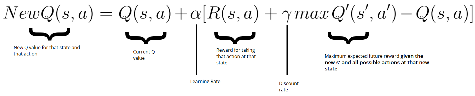
The bellman equation let’s us assess the q-value (quality) of a given state action pair. It states that the quality of taking an action at a given state, is equal to the immediate reward, plus the maximum discounted reward of the next state.</p>

<h3 id="qs-a--r--γ-maxₐqs-a">Q(s, a) = r + γ maxₐ’(Q(s’, a’))</h3>

<p>
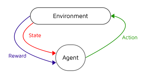
In other words, we’ll use a neural network to predict what action gives us the biggest future reward at any given state, by not only looking at the immediate state, but also, our prediction for the one that comes after it.</p>

<p>Initially, we know nothing about our game environment, so we need to explore it by making random moves and observing the outcome. After a while, we’ll start slowly moving away from this exploration approach and into an approach of exploiting our predictions, in order to improve them and win the game.</p>

<p>If we exploit too early, we won’t get chance to try new novel ideas which could improve our performance. If we explore too much, we won’t make progress. This is known as the exploration vs exploitation tradeoff.</p>

<h2 id="experience-replay">Experience Replay</h2>

<p>In our last post we introduced the concept of experience replay. Experience replay helps our network to learn from past actions. At each step, we’ll take our observation and append it to the end of a list (which we’ll call our ‘memory’). We implement the list as a deque in python, a double ended queue of fixed size that automatically removes the oldest element every time we add something new to the list. We’ll then feed this minibatch into our network to train our predictions of Q values. As our network improves, so do our experiences, which feeds back into our network.</p>

<p>Last time we used a relatively short memory, but this time, we’re going to store the last one million frames of gameplay.</p>

<h2 id="convnet">Convnet</h2>

<p>We’ll swap out our standard neural network for a convolutional neural network and learn to make decisions based on nothing but the raw pixel data of our game. This means that our agent will have to learn what is an enemy, what is a ball, what shooting does, and all other possible actions and consequences. The advantage of this is that we’re no longer tied to a game. Our agent will be able to learn a wide variety of Atari games based purely on pixel input.</p>

<p>Our convnet architecture if pretty standard, we’ll have three convolutional layers, a flatten layer, and two fully connected layers. The only difference is the we’ll omit the max pooling layers.</p>

<p>Max Pooling aims to make our network insensitive to small changes in the positions of features within our image. As our agent needs to know exactly where things are in our game, we’ll get rid of the traditional max pooling layers in our convnet all together.</p>

<h2 id="stacked-frames">Stacked Frames</h2>

<p>When we feed our frames into our convnet, we’ll actually use a stack of 4 frames. If you think about a single frame of a game of Pong, it’s impossible to know the direction the ball is going in or how fast. Using a stack of four frames gives us a sense of motion and speed that is necessary for our network to have the full picture. You can think of it like a mini video clip being fed to our network. Instead of our input being a single frame of the shape (105,80,1), we’ll now have four channels, taking the shape to (105,80,4).</p>

<h2 id="frame-skipping">Frame Skipping</h2>

<p>In their original paper, DeepMind skipped four frames every time they looped through gameplay. Their reasoning for doing this was that the environment doesn’t change much between single frames, we’d get a better representation of speed and movement by only looking at every fourth frame, plus we would reduce the amount of frame we need to process.</p>

<p>We’ll use frame skipping in our implementation, but how do we implement it? Fortunately this has been taken care of in OpenAI’s gym library.</p>

<hr />

<blockquote>
  <p><em>Maximize your score in the Atari 2600 game MsPacman. In this environment, the observation is an RGB image of the screen, which is an array of shape (210, 160, 3) Each action is repeatedly performed for a duration of kkk frames, where kkk is uniformly sampled from {2,3,4}{2, 3, 4}{2,3,4}.</em></p>
</blockquote>

<hr />

<p>The version number at the end of most games (<code>gym.make('MsPacman-v4')</code>) isn’t a version number at all, but refers to the amount of frames we skip. We can skip anywhere from no frames, to four frames by amending the number at the end of our environment name. For example…</p>

<ul>
  <li>MsPacman-v0 = No frame skipping</li>
  <li>MsPacman-v2 = Look at every second frame</li>
  <li>MsPacman-v3 = Look at every third frame</li>
  <li>MsPacman-v4 = Look at every fourth frame</li>
</ul>

<h2 id="performance">Performance</h2>

<p>Storing a million frames of pixels in memory can be quite computationally expensive. Our arrays for a single frame are 105 by 80 pixels, that’s 8400 pixels per frame. The numpy default array stores each of these pixels as a 32 bit float, meaning that our total memory (8400 * 32bits * 1000000) could take up to 33.6 gigabytes of RAM!</p>

<p>To combat this, we’ll specify our datatypes as uint8 for our frames and convert them to floats at the last minute before we feed them into our network. This will bring our RAM usage down from 33.6 to 8.4 gigabytes, much better!</p>

<h2 id="building-our-dqn">Building our DQN</h2>

<p>Let’s start by importing our dependencies…</p>

<pre><code class="language-python">import numpy as np
from keras import Sequential
from keras.layers import Dense, Flatten
from keras.layers.convolutional import Conv2D
from keras.optimizers import Adam
from keras.callbacks import ModelCheckpoint
from collections import deque
import gym
import random
</code></pre>

<p>Next we’ll define our DQNetwork class. I’ll keep indentation consistent, but I’ll break up some of the code so that we can walk through it block by block and really understand what’s happening.</p>

<pre><code class="language-python">class DQNetwork:
    def __init__(self, env):
        self.env              = env
        self.state_size       = env.observation_space.shape[0]
        self.action_size      = env.action_space.n
        self.memory           = deque(maxlen=1000000)
        self.stack            = deque([np.zeros((105,80), dtype=np.uint8) for i in range(4)], maxlen=4)
        self.gamma            = 0.9
        self.epsilon          = 1.0
        self.epsilon_min      = 0.01
        self.epsilon_decay    = 0.00003
        self.learning_rate    = 0.00025
        self.batch_size       = 64
        self.frame_size       = (105, 80)
        self.possible_actions = np.array(np.identity(self.action_size, dtype=int).tolist())
        self.model            = self.build_model()
</code></pre>

<p>Our <code>__init__</code> method is mostly the same as our last model. We’re setting up some key parameters to use later, like our gamma, epsilon (exploration vs exploitation trade off), our deque for our memory, and building and storing our model.</p>

<p>The new things are…</p>

<ul>
  <li><code>stack</code> - A smaller deque to help stack our four frames together to show our network a sense of motion</li>
  <li><code>possible_actions</code> - One hot encoded list of our possible actions (will come in handy later)</li>
  <li><code>frame_size</code> - The size of our preprocessed frames. It makes sense to abstract this out as we’ll be typing this a lot</li>
</ul>

<p>
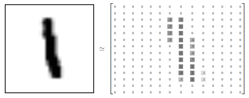
Next we’ll need to think about preprocessing our frames before feeding them into our network. We’ll greyscale them as colour doesn’t add any additional information to our network and would take up three times the space (red, green and blue channels as opposed to a single greyscale channel). Notice we’re storing our frames as uint8 and not normalizing our frames to be between 0-1 (which we would traditionally do to prepare our data for our network). Instead, we’ll normalize on demand later on to save memory.</p>

<pre><code class="language-python">    def preprocess_frame(self, frame):
        """Resize frame and greyscale, store as uint8 and normalize on demand to save memory"""
        frame = frame[::2, ::2]
        return np.mean(frame, axis=2).astype(np.uint8)
</code></pre>

<p>We’ll also need a method to append a frame to the end of our four frame stack deque that we defined earlier. Our deque will handle removing the oldest frame, but there is an exception that we need to handle. At the beginning of our game, we’ll need to stack the same frame four times to fill out our stack. We’ll have our method take an optional <code>reset=True</code> parameter that clears the stack and adds the same frame four times. Our final stacked state that we pass into our network will end up being of the shape (105,80,4).</p>

<pre><code class="language-python">    def append_to_stack(self, state, reset=False):
        """Preprocesses a frame and adds it to the stack"""
        frame = self.preprocess_frame(state)

        if reset:
            # Reset stack
            self.stack = deque([np.zeros((105,80), dtype=np.int) for i in range(4)], maxlen=4)

            # Because we're in a new episode, copy the same frame 4x
            for i in range(4):
                self.stack.append(frame)
        else:
            self.stack.append(frame)

        # Build the stacked state (first dimension specifies different frames)
        stacked_state = np.stack(self.stack, axis=2)

        return stacked_state
</code></pre>

<p>We’ll need to create a similar method to store our experiences in memory, and retrieve a random minibatch…</p>

<pre><code class="language-python">    def remember(self, state, action, reward, new_state, done):
        self.memory.append((state, action, reward, new_state, done))

    def memory_sample(self, batch_size):
        """Sample a random batch of experiences from memory"""
        memory_size = len(self.memory)
        index       = np.random.choice(np.arange(memory_size), size=batch_size, replace=False)
        return [self.memory[i] for i in index]
</code></pre>

<p>
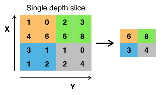
Next, we’ll build our model. This is almost identical as last time, except that we’re using the Conv2D layer from Keras, and exclusing the traditional max pooling layer that we’d normally add with a convolutional network. (Remember, max pooling makes our network insensitive to position changes. Great for object detection and classification, but not great when our game depends on the position of the features we detect!)</p>

<pre><code class="language-python">    def build_model(self):
        """Build the neural net model"""
        model = Sequential()
        model.add(Conv2D(32, (8, 4), activation='elu', input_shape=(105, 80, 4)))
        model.add(Conv2D(64, (3, 2), activation='elu'))
        model.add(Conv2D(64, (3, 2), activation='elu'))
        model.add(Flatten())
        model.add(Dense(512, activation='elu', kernel_initializer='glorot_uniform'))
        model.add(Dense(self.action_size, activation='softmax'))
        model.compile(loss='mse', optimizer=Adam(lr=self.learning_rate))
        return model
</code></pre>

<p>Our agent will need to be able to make two types of move, depending on where we are in our exploration vs exploitation journey. We’ll write a method that returns a random action, and a method which takes in our state (105,80,4), and predicts the best action (according to our neural network).</p>

<p>Notice in the <code>predict_action</code> method, we first divide by 255 to normalize our values between 0 and 1. Secondly, we’ll reshape our state from (105,80,4), to (1,105,80,4), a necessary step for keras to consume our data. You can think of our shape like this: (number of examples, height, width, depth). Our network will return a vector the size of our possible actions, from which, we’ll return the index of the action we predicted, ready to feed into our <code>env.step</code> call.</p>

<pre><code class="language-python">    def random_action(self):
        """Returns a random action"""
        return random.randint(1,len(self.possible_actions)) - 1

    def predict_action(self, state):
        """Returns index of best predicted action"""
        state  = state / 255
        state  = state.reshape((1, *state.shape)) # Reshape our state to a single example for our neural net
        choice = self.model.predict(state)
        return np.argmax(choice)
</code></pre>

<p>With our <code>random_action</code> and <code>predict_action</code> methods defined, we can now write a function to select which one to choose depending on where we are on our explore vs exploit spectrum.</p>

<p>We’ll also use a slightly different way of calculating our explore vs exploit probability depending on the step in our game play. Lastly, we’ll return our <code>explore_probability</code> to log out later.</p>

<pre><code class="language-python">    def select_action(self, state, decay_step):
        """Returns an action to take with decaying exploration/exploitation"""

        explore_probability = self.epsilon_min + (self.epsilon - self.epsilon_min) * np.exp(-self.epsilon_decay * decay_step)

        if explore_probability &gt; np.random.rand():
            # Exploration
            return self.random_action(), explore_probability
        else:
             # Exploitation
            return self.predict_action(state), explore_probability
</code></pre>

<h2 id="training">Training</h2>

<p>With the majority of our agent built, there’s only one more method to implement; training our model with experiences from our replay memory.</p>

<p>Firstly, we’ll check to see if our memory is less than our batch size of 64. If we don’t have enough experiences logged yet, we’ll exit the function and let our agent keep gathering random experiences until we have enough experience to form a complete minibatch to train on.</p>

<p>Next we prepare our minibatch. First we’ll select a random minibatch of 64 experiences, notice we also divide our <code>states_mb</code> and <code>next_states_mb</code> by 255 to normalise our frames to be between 0 and 1. Next, we’ll grab our predictions for our current state (shape (64, 105, 80, 4)), as well as the predictions for our next states.</p>

<p>With our predictions, we can assemble a corresponding list of the Q-values for each state. If we’ve reached a terminal state, and the game is over, then our Q-value is equal to the final reward (as there are no more future rewards). If we’ve not yet reached the end of our game, then our Q-value is set to the immediate reward (from the <code>rewards_mb[i]</code> list, plus the maximum discounted future reward (gamma * the maximum reward from our next state prediction).</p>

<p>Once we’ve finished our corresponding Q-values list, we can fit our model for one epoch, with our <code>states_mb</code> as our input, and our <code>targets_mb</code> as our labels. A single iteration doesn’t seem much here, but remember we’ll be calling this replay method at every step throughout our gameplay.</p>

<pre><code class="language-python">   def replay(self):
        if len(self.memory) &lt; self.batch_size:
            return

        # Select a random minibatch from memory
        minibatch = self.memory_sample(self.batch_size)

        # Split out our tuple and normalise our states
        states_mb      = np.array([each[0] for each in minibatch]) / 255
        actions_mb     = np.array([each[1] for each in minibatch])
        rewards_mb     = np.array([each[2] for each in minibatch])
        next_states_mb = np.array([each[3] for each in minibatch]) / 255
        dones_mb       = np.array([each[4] for each in minibatch])

        # Get our predictions for our states and our next states
        target_qs         = self.model.predict(states_mb)
        predicted_next_qs = self.model.predict(next_states_mb)

        # Create an empty targets list to hold our Q-values
        target_Qs_batch = []

        for i in range(0, len(minibatch)):
            done = dones_mb[i]

            if done:
                # If we finished the game, our q value is the final reward (as there are no more future rewards)
                q_value = rewards_mb[i]
            else:
                # If we havent, our q value is the immediate reward, plus future discounted reward (gamma is our discount)
                q_value = rewards_mb[i] + self.gamma * np.max(predicted_next_qs[i])

            # Fit target to a vector for keras (represent actions as one hot * q value (q gets set at the action we took, everything else is 0))

            one_hot_target = self.possible_actions[actions_mb[i]]
            target         = one_hot_target * q_value
            target_Qs_batch.append(target)

        targets_mb = np.array([each for each in target_Qs_batch])

        self.model.fit(states_mb, targets_mb, epochs=1, verbose=1) # Change to verbose=0 to disable logging
</code></pre>

<h2 id="training-our-dqn">Training our DQN</h2>

<p>With our DQNetwork class complete, we just need to train our model. As we’ve dramatically increased our state space, our model is going to take quite a long time to train. We’re training for around 2.5 million frames of game play (50 episodes, each with a maximum of 50,000 steps per game), a conventional laptop isn’t going to cut it here (unless you’ve got a lot of RAM and are happy to leave it running for a week or two!).</p>

<p>I’ve included a section about my recommendations for training on an AWS instance below. But first, let’s talk about what’s happening in our training loop.</p>

<p>We’ll start by initialising our environment, as well as a monitor wrapper which will record each episode to video for us to review later. We’ll loop through our episodes, taking a maximum of 50000 steps per game.</p>

<p>At each step, we’ll pick an action based on exploration/exploitation and observe the reward and new state. We’ll append these to our memory, as we’ll need them to train on later.</p>

<p>If it turns out we’ve finished our game and are at the terminal state, we’ll create a blank frame to represent our <code>next_state</code> add to our stack. This let’s us record the final reward, if we didn’t stack a blank frame, we’d lose all the information and rewards we were awarded at the final state.</p>

<p>If we’re still playing our game, we’ll add our frame to the end of our four frame stack, set the <code>state</code> equal to the <code>next_state</code> to move the game on, and train our agent on a random minibatch of 64 previous experiences.</p>

<pre><code class="language-python">env         = gym.make('Pong-v4')
env         = gym.wrappers.Monitor(env, './videos/', video_callable=lambda episode_id: True) # Save each episode to video
agent       = DQNetwork(env)
episodes    = 50
steps       = 50000
decay_step  = 0

for episode in range(episodes):
    episode_rewards = []

    # 1. Reset the env and frame stack
    state         = agent.env.reset()
    state         = agent.append_to_stack(state, reset=True)

    for step in range(steps):
        decay_step += 1

        # 2. Select an action to take based on exploration/exploitation
        action, explore_probability = agent.select_action(state, decay_step)

        # 3. Take the action and observe the new state
        next_state, reward, done, info = agent.env.step(action)

        # Store the reward for this move in the episode
        episode_rewards.append(reward)

        # 4. If game finished...
        if done:
            # Create a blank next state so that we can save the final rewards
            next_state = np.zeros((210,160,3), dtype=np.uint8)
            next_state = agent.append_to_stack(next_state)

            # Add our experience to memory
            agent.remember(state, action, reward, next_state, done)

            # Save our model
            agent.model.save_weights("model-ep-{}.h5".format(episode))

            # Print logging info
            print("Game ended at episode {}/{}, total rewards: {}, explore_prob: {}".format(episode, episodes, np.sum(episode_rewards), explore_probability))
            # Start a new episode
            break
        else:
            # Add the next state to the stack
            next_state = agent.append_to_stack(next_state)

            # Add our experience to memory
            agent.remember(state, action, reward, next_state, done)

            # Set state to the next state
            state = next_state

        # 5. Train with replay
        agent.replay()
</code></pre>

<h2 id="training-on-ec2">Training on EC2</h2>

<p>I opted to train my model using a p2.xlarge instance on EC2. I ran the code as a regular python file, within a tmux session. That way I could detatch from the session and it would keep running. If you were to try running this inside a Jupyter notebook, the code would stop running as soon as you closed your browser or laptop, given that this can take days or weeks to train, it’s best to have an environment you can completely detatch from and come back to later.</p>

<p>You can follow this tutorial to get Jupyter Notebook up and running on an EC2 instance with GPU (follow up to the jupyter part to get your EC2 instance running):</p>

<p><a href="https://medium.com/@margaretmz/setting-up-aws-ec2-for-running-jupyter-notebook-on-gpu-c281231fad3f">https://medium.com/@margaretmz/setting-up-aws-ec2-for-running-jupyter-notebook-on-gpu-c281231fad3f</a></p>

<p>Once you’ve set up your EC2 instance, you’ll need to ssh into your instance, install some dependencies and download the roms for the Atari games…</p>

<pre><code>sudo apt install unrar
sudo apt install ffmpeg
</code></pre>

<p>Download and import Atari roms…</p>

<pre><code>wget http://www.atarimania.com/roms/Roms.rar
unrar x Roms.rar &amp;&amp; unzip Roms/ROMS.zip
pip install gym gym-retro gym[atari]
python -m retro.import ROMS/
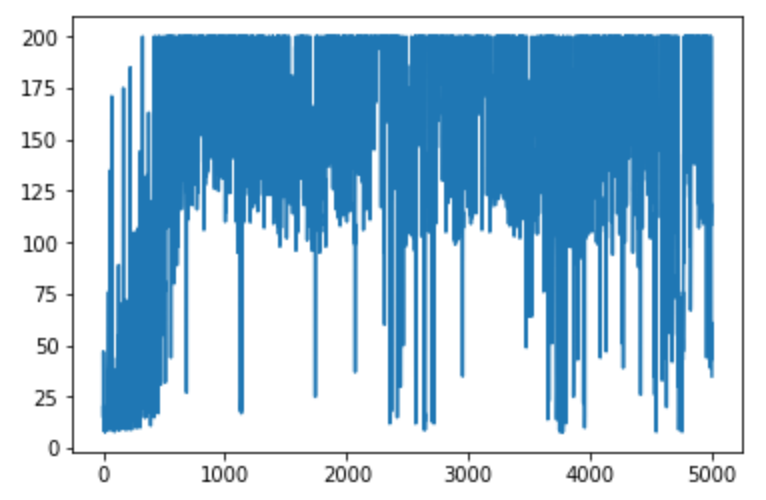
</code></pre>

<h2 id="results">Results</h2>

<p>Here’s Playing at episode 1. Some times we’ll hit the ball accidentally, but we’re still in the explore phase, so a lot of our movement is random and jittery.</p>

<p><img src="/assets/images/deep_q_learning_for_atari_games/pong_ep_1.gif" alt="Pong at episode one" /></p>

<p>Updates coming over the next few days as training completes!</p>

<h2 id="resources">Resources</h2>

<p>Here are a couple of articles that really helped me with wrapping my head around the implementation of this…</p>

<p><a href="https://ai.intel.com/demystifying-deep-reinforcement-learning/#gs.AfY3CNJe">https://ai.intel.com/demystifying-deep-reinforcement-learning/#gs.AfY3CNJe</a></p>

<p><a href="https://becominghuman.ai/lets-build-an-atari-ai-part-1-dqn-df57e8ff3b26">https://becominghuman.ai/lets-build-an-atari-ai-part-1-dqn-df57e8ff3b26</a></p>

<p><a href="https://medium.com/@margaretmz/setting-up-aws-ec2-for-running-jupyter-notebook-on-gpu-c281231fad3f">https://medium.com/@margaretmz/setting-up-aws-ec2-for-running-jupyter-notebook-on-gpu-c281231fad3f</a></p>]]></content><author><name>Spencer Dixon</name></author><category term="deep-learning" /><category term="q-learning" /><category term="reinforcement-learning" /><category term="atari" /><category term="python" /><summary type="html"><![CDATA[Build an AI agent that learns to play Space Invaders and other Atari games. Combine Deep Q-Networks with CNNs to learn directly from game screen pixels using OpenAI Gym.]]></summary></entry><entry><title type="html">A Primer on Reinforcement Learning: Q-Learning</title><link href="https://spencer.wtf/2018/11/01/a-primer-on-reinforcement-learning.html" rel="alternate" type="text/html" title="A Primer on Reinforcement Learning: Q-Learning" /><published>2018-11-01T10:43:00+00:00</published><updated>2018-11-01T10:43:00+00:00</updated><id>https://spencer.wtf/2018/11/01/a-primer-on-reinforcement-learning</id><content type="html" xml:base="https://spencer.wtf/2018/11/01/a-primer-on-reinforcement-learning.html"><![CDATA[<p>Reinforcement Learning is a field of Machine Learning which aims to develop intelligences that learn through trial and error by exploring and interacting with their environment.</p>

<p>You may have seen exciting demos of an AI learning to play video games or robot arms learning to manipulate objects or mimic tasks.</p>

<p>In this post, we’ll look at a very basic approach to Reinforcement Learning which we can use to learn to play very simple games. It’s a limited approach and we’ll quickly find problems with it, but that will set us up nicely for a follow up post on how we can improve on this technique</p>

<h2 id="state-actions-and-rewards">State, Actions and Rewards</h2>

<p>Reinforcement Learning (RL) consists of two actors: an agent (our model / algorithm), and the environment (the game we’re playing in this case). Our agent seeks to develop an optimal policy for interacting with the environment that maximises the cumulative reward over time.</p>

<p>Our environment is represented by a series of <em>states</em>. If we think of a grid with a single playing piece, we can transition states by moving our piece around the board. Each move takes us to a different possible state that the game can be in. We have several different things we can do to our piece, known as <em>actions</em>. We can move up, down, left, or right. Each of these actions transitions us to a new state and brings us one step closer to, or further away from, our goal state (usually a state that will win the game).</p>

<p>When we take an action in our game, we receive some feedback, usually in the form of a score. It’s this <em>reward</em> that we seek to maximise over our time playing the game.</p>

<p>In short, our agent interacts with our environment by choosing <em>actions</em> (a) to take at a particular <em>state</em> (s) with the intention of maximising future <em>rewards</em> (r) received. It’s this mapping of what action we should take at what particular state that’s the problem that we need to solve and is referred to as the <em>policy</em> (π), with the optimal policy being denoted as <em>π&amp;ast;</em></p>

<p><img src="/assets/images/a_primer_on_reinforcement_learning/cycle.png" alt="The Reinforcement Learning Cycle" /></p>

<h2 id="the-q-table">The Q-Table</h2>

<p>There are a lot of different techniques that we can use to get our model to converge on an optimal policy but in this post, we’re going to go for the one which allows us to get something up and running quickly.</p>

<p>Q-Learning is a technique that seeks to assess the <em>quality</em> of taking a given action at a given state. If we drew up a table, with all our game states as rows, and all our possible actions as columns. We could use it as a cheat sheet to keep track of the rewards we recieve for a state action pair over time. If we move left at state 1, and receive a reward of +1, we’ll write that down in our table. Over time, we’ll begin to build up a picture of the quality of every action we can take at every state, and could easily select the actions with the biggest score, or Q-value, to cheat our way to the end of the game.</p>

<p>But this raises two important questions, how do we update our score for each state action pair? And, how do we move around our game when we have no values in our table yet?</p>

<h2 id="the-bellman-equation">The Bellman Equation</h2>

<p>The Bellman Equation provides the foundation for assessing the quality of taking a given action at a given state. If we know the rewards at each state in the game, for example, landing on a safe tile is +1 point, and losing the game is -10 points, we can use the Bellman equation to calculate the optimal Q-value for each state action pair.</p>

<p>We’ll iteratively update our Q-values in our Q-table until we converge to the optimal policy, seeking to reduce the loss between our Q-value, and our optimal Q-value.</p>

<p>Firstly, we’ll need to take an action from our state. Then we’ll receive our reward, along with a new state. We can use this new information, along with the information of the action we took at the previous state to assess how good or bad our move was.</p>

<p>What if we come across a reward for a state action pair we’ve already seen? Over writing previous Q-values would lose valuable information about previous game plays. Instead, we can use a learning rate to update our Q-value. The higher the learning rate, the more quickly our agent will adopt new values and disregard previous values. With a learning rate of 1.0, our agent would simply rewrite all the old values with new values each time.</p>

<p><img src="/assets/images/a_primer_on_reinforcement_learning/bellman.png" alt="The Bellman Equation" /></p>

<h2 id="exploration-vs-exploitation">Exploration vs Exploitation</h2>

<p>Imagine our agent is playing a game with an empty Q table. Initially, it’ll be fairly useless, so using it as a policy to follow won’t get us anywhere. In fact, when we do build up values in our Q table, we’ll want to avoid using them too early before they’ve converged. If we exploit our table too soon, we’ll get stuck at early rewards and possibly miss out on taking larger rewards that could benefit us long term.</p>

<p>Instead, we’ll want to strike a decaying balance between how much we want to explore the games state spaces to find new rewards, and how much we want to exploit our Q table for the correct answers. This is referred to as exploration vs exploitation.</p>

<p>We’ll do this with a strategy known as <em>epsilon greedy</em>. We’ll set an <code>epsilon</code> number, which represents our probability of choosing exploration vs exploitation. With epsilon set to 1.0, we have a 100% chance that we’ll explore our environment, and thus take actions entirely at random. With epsilon at 0, we’ll exploit our Q-table and select the action with the highest value. As we iterate through our training, we’ll slowly decay epsilon by <code>gamma</code>, a small number, that will make it less and less probable over time that we’ll explore our environment by selecting random actions.</p>

<h2 id="frozen-lake">Frozen Lake</h2>

<p>Frozen Lake is a game where we have to navigate a 4x4 grid of tiles, each of a different surface type. S is our starting point, G is our goal point, F are frozen tiles (safe to step on) and H are holes which we can fall into and lose the game. We’ll train an agent to safely navigate from the starting tile to our goal tile using Q-Learning.</p>

<pre><code class="language-python">SFFF
FHFH
FFFH
HFFG
</code></pre>

<p>We’ll first import OpenAI’s gym library, which will give us the FrozenLake game, with a nice wrapper to be able to access actions and the state space. We’ll also require numpy and random.</p>

<pre><code class="language-python">import numpy as np
import random
import gym
</code></pre>

<p>Next we’ll start up our FrozenLake game and assign the environment to a variable we can use later on</p>

<pre><code class="language-python">env = gym.make("FrozenLake-v0")
</code></pre>

<p>In order to form our Q table, we’ll need to know the number of possible actions and states. We’ll then create an empty table, initialised with zeros at the moment, that we can later update throughout our training with our Q values, much like how we update weights in a neural network. Our Q table acts like a cheat sheet, reflecting the quality of taking that particular action, at a particular state.</p>

<pre><code class="language-python">action_size = env.action_space.n
state_size = env.observation_space.n

qtable = np.zeros((state_size, action_size))
print(qtable)
</code></pre>

<pre><code class="language-python">[[0. 0. 0. 0.]
 [0. 0. 0. 0.]
 [0. 0. 0. 0.]
 [0. 0. 0. 0.]
 [0. 0. 0. 0.]
 [0. 0. 0. 0.]
 [0. 0. 0. 0.]
 [0. 0. 0. 0.]
 [0. 0. 0. 0.]
 [0. 0. 0. 0.]
 [0. 0. 0. 0.]
 [0. 0. 0. 0.]
 [0. 0. 0. 0.]
 [0. 0. 0. 0.]
 [0. 0. 0. 0.]
 [0. 0. 0. 0.]]
</code></pre>

<p>Let’s set some hyperparameters…</p>

<pre><code class="language-python">episodes       = 10000      # Total episodes
max_steps      = 99         # Max moves per episode - stops us exploring infinitely

learning_rate  = 0.8        # Learning rate
gamma          = 0.95       # Discounting rate

epsilon        = 1.0        # Exploration vs exploitation rate
decay_rate     = 0.001      # How much we want to decay our exploration vs exploitation rate
</code></pre>

<p>We’ll write some helper functions that will make it easier to understand what our code is doing without getting caught up in the formulas.</p>

<p>Firstly, we’ll need a function that, over time, will make a gradual progression from exploration of our environment, to exploitation by utilising our Q table. We’ll use epsilon to denote our exploration vs exploitation rate, and reduce it by our <code>decay_rate</code> for every episode.</p>

<p><code>max_epsilon</code> is the largest our epsilon can be and represents a full 100% chance we’ll explore our environment. Conversely, <code>min_epsilon</code> represents a 100% chance that we’ll exploit our Q table for the correct answers.</p>

<pre><code class="language-python">def reduce_epsilon(episode, min_epsilon=0.01, max_epsilon=1.0, decay_rate=0.001):
    return min_epsilon + (max_epsilon - min_epsilon) * np.exp(-decay_rate * episode)
</code></pre>

<p>Epsilon will be used in selecting wether we want to explore our environment, which we’ll do by selecting an action at random, or wether we want to exploit our learned Q-table, which we can do by selecting the action with the highest Q value.</p>

<p>Since this is fairly simply logic, we can code this into another helper function which will help simplify our code…</p>

<p>Here we take in some information like our <code>epsilon</code>, our <code>qtable</code>, <code>state</code> and the <code>env</code> (environment) and generate a random number. If our number is larger than epsilon, we’ll choose to exploit our Q-table by selecting the action with the highest Q-value. If our number is lower than epsilon, we’ll explore our environment further by selecting a random action from our action space.</p>

<pre><code class="language-python">def select_action(epsilon, qtable, state, env):
    x = random.uniform(0,1)

    if x &gt; epsilon:
        # Exploitation
        return np.argmax(qtable[state,:])
    else:
        # Exploration
        return env.action_space.sample()
</code></pre>

<p>Lastly, we’ll need a function to update the values in our Q-table based upon the Bellman equation given our previous state, action taken, reward, and new state…</p>

<pre><code class="language-python">def update_qtable(qtable, state, action, reward, new_state, learning_rate, gamma):
    # Update Q(s,a):= Q(s,a) + lr [R(s,a) + gamma * max Q(s',a') - Q(s,a)]
    # qtable[new_state,:] : all the actions we can take from new state

    qtable[state, action] = qtable[state, action] + learning_rate * (reward + gamma * np.max(qtable[new_state, :]) - qtable[state, action])
    return qtable
</code></pre>

<h2 id="training-our-q-table">Training our Q-Table</h2>

<p>Next up is the bulk of our code. This is where we’ll put the pieces together, train our agent, and populate our Q-table.</p>

<p>For every episode in our total number of <code>episodes</code>, we’ll firstly reset our environment and a few variables which will keep track of game play for that particular run. For each step, we’ll use our <code>select_action()</code> function to choose an action, either at random (exploration) or from our Q-table (exploitation). This rate will gradually ramp towards more and more exploitation over time as we build up our Q-table.</p>

<p>We’ll then take our action and observe the reward and new state returned, which we’ll use to update our Q-table. Finally, we’ll we’ll set our <code>state</code> to be the <code>new_state</code> that we received by taking an action, reduce <code>epsilon</code> to lean slightly more towards exploitation, add our reward to a list so that we can keep track of how we’re improving over time, and start the cycle over again until we reach some terminal state in our game (we fall into a hole, or win the game).</p>

<pre><code class="language-python">rewards = []

for episode in range(episodes):
    # Reset the environment
    state = env.reset()
    step = 0
    done = False
    total_rewards = 0

    for step in range(max_steps):
        # Use epsilon to pick an action, either at random, or from our q-table
        action = select_action(epsilon, qtable, state, env)

        # Take the action and observe the new state and reward
        new_state, reward, done, info = env.step(action)

        # Update our Q-table to take note of how valuable the action according to the reward we got
        qtable = update_qtable(qtable, state, action, reward, new_state, learning_rate, gamma)

        # Set state to the new state we received (where we moved to)
        state = new_state

        total_rewards += reward

        # If the game is over, exit the loop, back to a new training loop
        if done == True:
            break

        epsilon = reduce_epsilon(episode)

    rewards.append(total_rewards)

print("Score over time: " +  str(sum(rewards)/total_episodes))
print(qtable)
</code></pre>

<h2 id="playing-the-game">Playing the Game</h2>

<p>Once we’ve populated our Q-table, we can exploit it to play the game successfully. As we’re simply following our Q-table, we no longer have to deal with updating our table, or dealing with our exploration vs exploitation trade off. We can simply just follow the policy of selecting the highest value at a given state. With a well trained Q-table, our values should closely reflect the maximum expected reward over time by taking that particular action at that particular state.</p>

<pre><code class="language-python">env.reset()

for episode in range(5):
    state = env.reset()
    step = 0
    done = False
    print("Playing Round #", episode)

    for step in range(max_steps):
        # Select the action with the highest reward
        action = np.argmax(qtable[state,:])

        # Return our new state and reward
        new_state, reward, done, info = env.step(action)

        if done:
            # If the game is finished, we'll print our environment to see if we fell into a hole, or ended on our goal tile
            env.render()

            # We print the number of steps it took.
            print("Steps taken:", step)
            break

        state = new_state

env.close()
</code></pre>

<h2 id="summary">Summary</h2>

<p>And there we have it! We successfully trained a model to learn play the Frozen Lake game by exploring the environment itself, and learning through trial and error.</p>

<p>But what happens when we want to play a more complex game with millions of possible states? Unfortunately, as your state space grows, you very quickly out grow the feasibility of using a Q-table. It would take millions of iterations to even begin to explore all the possible state spaces and build up an accurate Q-table.</p>

<p>Instead of creating a cheat sheet that we can look up every possible value for every possible action in every possible state, what if we could just simplify by having a function that approximates the Q-value for a given state action pair?</p>

<p>If you have read previous posts, you may be familiar with one tool that we can use for function approximation; the neural network.</p>

<p>In a future post we’ll look at how we can improve on our reinforcement learning agent by using neural networks to apply our techniques to larger state spaces and more complex games with Deep Q-Learning.</p>]]></content><author><name>Spencer Dixon</name></author><category term="machine-learning" /><category term="reinforcement-learning" /><category term="q-learning" /><category term="python" /><summary type="html"><![CDATA[Introduction to reinforcement learning and Q-Learning. Learn about states, actions, rewards, and the Bellman equation through building an AI that learns to play simple games.]]></summary></entry><entry><title type="html">We need to go deeper: Deep Q Networks</title><link href="https://spencer.wtf/2018/11/01/we-need-to-go-deeper-deep-q-networks.html" rel="alternate" type="text/html" title="We need to go deeper: Deep Q Networks" /><published>2018-11-01T10:43:00+00:00</published><updated>2018-11-01T10:43:00+00:00</updated><id>https://spencer.wtf/2018/11/01/we-need-to-go-deeper-deep-q-networks</id><content type="html" xml:base="https://spencer.wtf/2018/11/01/we-need-to-go-deeper-deep-q-networks.html"><![CDATA[<p>In the last post we looked at Q-Learning with respect to reinforcement learning; the idea that we can assess the quality of a particular state action pair and build up a cheat sheet that allows us to play the game proficiently.</p>

<p>Unfortunately we quickly came to the bottleneck in this problem; that as our state space grows, it becomes more and more computationally expensive to calculate the quality for every possible state action pair (that coupled with the fact that this only works on an environment that can be modelled with a Markov Decision Process). Instead of creating a Q-table (check out the previous post if you’re not familiar with Q-tables), we need a way to approximate the quality of an action without storing every possible combination of state action pairs.</p>

<p>Enter the good old neural network.</p>

<p>A neural network works like a blank brain that you can train to associate some input with some output. Give it 10,000 images of cats and dogs, along with the correct answers, and it will map the input to the output and be able to classify cat or dog on a new image that it hasn’t seen before. The caveat here is that you need to provide the correct answers during training. This means neural networks are a <em>supervised</em> learning problem.</p>

<p>Mathematically, we’re simply seeking to minimise the difference between the predictions from our neural net, and the actual correct answers. As long as there is a small error, our neural net will, on average, predict the same thing as the correct answer.</p>

<p>Enter our game for this post and our loss function…</p>

<h2 id="learning-to-play-cartpole">Learning to play CartPole</h2>

<p>Cart Pole is a game which ships with OpenAI’s gym library for reinforcement learning. It consists of a pole, hinged on a movable cart. The objective is simple; move the cart left or right to keep the pole balanced and upright.</p>

<p><img src="/assets/images/we_need_to_go_deeper/cartpole.gif" alt="Cartpole" /></p>

<p>But there’s a problem. With reinforcement learning, we seek to maximise our cumulative rewards over time. If we received a reward for moving the cart to the right to retain balance of the pole, then we may try moving the cart right again to get another reward. This unwanted behaviour is rampant in reinforcement learning and demonstrates how a simple oversight can turn good AI bad.</p>

<p>Instead of maximising reward, we want to maximise time. Our agent’s goal will be to keep the game going for as long as possible.</p>

<h2 id="experience-replay">Experience Replay</h2>

<p>Imagine we’re playing a game where our enemy pops out at either the right, or left of the screen. Each round is random, but suppose we get a large amount of rounds that favour one particular side. As our agent is trained sequentially, our neural net begins to favour that particular side and develops a bias in its prediction of future actions. In other words, we start to favour recent data and forget past experiences.</p>

<p>How do we train our neural net in a way that it doesn’t favour what it’s recently learned? How do we prevent our neural net from forgetting past experiences that may be relevant in the future?</p>

<p>The answer is surprisingly simple. We introduce the concept of experience replay, or memory. Every time we are exposed to a state action pair, we’ll store it away in an special python list type called a <code>deque</code> (it’s essentially a list of a fixed size, that removes the oldest element each time that you add a new one to it. That way we’ll have a constantly updating buffer of the last <code>n</code> number of state action pairs to train from).</p>

<p>With our experience replay buffer built up, we can randomly sample minibatches of experiences to train from and benefit from a wider look at our environment. Additionally, as our neural net gets better, so do the state action pairs that we train our neural net from. It’s a win win.</p>

<h2 id="building-the-cartpole-agent">Building the CartPole Agent</h2>

<p>We’ll start by importing our dependencies. Most of it is the same as last time, but we’ll use Keras for our neural net, and matplotlib for plotting our score over time.</p>

<pre><code class="language-python">import numpy as np
import gym
from keras import Sequential
from keras.layers import Dense
from keras.optimizers import Adam
import matplotlib.pyplot as plt
from collections import deque
</code></pre>

<p>Next, we’ll build our agent. Note that this is all one class but I’ll try to break it up and talk about each method. Pay particular notice to the indentation here.</p>

<p>Our agent will take in the environment and hold the hyperparameters. We’ll use the <code>env</code> argument to determine our state size and action size.</p>

<pre><code class="language-python">class Agent:
    def __init__(self, env):
        self.memory        = deque(maxlen=600)
        self.state_size    = env.observation_space.shape[0]
        self.action_size   = env.action_space.n
        self.gamma         = 0.95    # discount rate
        self.epsilon       = 1.0     # exploration rate
        self.epsilon_min   = 0.01
        self.epsilon_decay = 0.995
        self.learning_rate = 0.001
        self.model         = self.build_model()
</code></pre>

<p>Notice in the initialisation of our agent, we made a call to a <code>build_model()</code> method. Let’s write that now to return our neural net from Keras. We’ll store this in a hyperparam so that we can make calls to predict actions or train it later.</p>

<pre><code class="language-python">    def build_model(self):
        model = Sequential()
        model.add(Dense(24, input_dim=self.state_size, activation='relu'))
        model.add(Dense(24, activation='relu'))
        model.add(Dense(self.action_size, activation='linear'))
        model.compile(loss='mse', optimizer=Adam(lr=self.learning_rate))
        return model
</code></pre>

<p>Much like our previous tutorial, we’ll need a way to select an action based on our exploration / exploitation trade off. We’ll choose a random number between 1 and 0. If our number is greater than epsilon, we’ll use our neural net to predict which action we should take (exploitation), if it’s lower, we’ll select and action at random and continue to explore our environment.</p>

<pre><code class="language-python">    def select_action(self, state):
        # Selects an action based on a random number
        # If the number is greater than epsilon, we'll take the predicted action for this state from our neural net
        # If not, we'll choose a random action
        # This helps us navigate the exploration/exploitation trade off
        x = np.random.rand()

        if x &gt; self.epsilon:
            # Exploitation
            actions = self.model.predict(state)
            return np.argmax(actions[0])
        else:
            # Exploration
            return random.randrange(self.action_size)
</code></pre>

<p>Next we’ll introduce the idea of experience replay. We’ll write a very simple function that takes the <code>state</code>, <code>action</code>, <code>reward</code>, <code>next_state</code>, <code>done</code> data returned from taking an action on our environment, and adds it to the end of our deque (removing the oldest element at the same time)…</p>

<pre><code class="language-python">    def remember(self, state, action, reward, next_state, done):
        self.memory.append((state, action, reward, next_state, done))
</code></pre>

<p>Lastly, we’ll need a function to train our neural net from our experience replay buffer. Firstly, we’ll make sure that we have enough experiences in our buffer to train from. If we don’t we’ll simply exit the function and keep exploring our environment until we do.</p>

<p>When we have enough experiences to sample from, we’ll take a random sample of experiences which we’ll call our minibatch, and use that to train the network by calculating our predicted Q-values.</p>

<p>Finally, we’ll reduce our epsilon to gradually nudge us more and more towards exploitation of our neural net in prediction our Q value, rather than exploring our environment by taking random actions.</p>

<pre><code class="language-python">    def train_with_replay(self, batch_size):
        # If we dont have enough experiences to train, we'll exit this function
        if len(self.memory) &lt; batch_size:
            return
        else:
            # Sample a random minibatch of states
            minibatch = random.sample(self.memory, batch_size)

            # For each var in the minibatch, train the network...
            for state, action, reward, next_state, done in minibatch:
                # If we haven't finished the game, calculate our discounted, predicted q value...
                if not done:
                    q_update_target = reward + self.gamma * np.amax(self.model.predict(next_state)[0])
                else:
                    # If we have finished the game, our q-value is our final reward
                    q_update_target = reward

                # Update the predicted q-value for action we tool
                q_values            = self.model.predict(state)
                q_values[0][action] = q_update_target

                # Train model on minibatches from memory
                self.model.fit(state, q_values, epochs=1, verbose=0)

                # Reduce epsilon
                if self.epsilon &gt; self.epsilon_min:
                    self.epsilon *= self.epsilon_decay
</code></pre>

<h2 id="training-our-deep-q-network">Training our Deep Q-Network</h2>

<p>With our agent written, we’ll piece everything together and start training our deep Q-network. We’ll start by defining our cart pole environment and setting our environment specific hyperparameters like number of episodes and minibatch size. We’ll also keep track of our scores in an array in order to graph them out at the end.</p>

<pre><code class="language-python">env        = gym.make('CartPole-v0')
episodes   = 5000
max_steps  = 200
batch_size = 32
agent      = Agent(env)
scores     = []
</code></pre>

<p>We’ll loop through our total number of episodes, and, in a smaller loop, step through our environment, taking actions and observing their rewards. We’ll add our observation to the experience replay buffer. At the end of our game, we’ll print our score, and train our agent on a random minibatch of experiences at the end of each episode.</p>

<pre><code class="language-python">for episode in range(episodes):
    # Reset the environment
    state = env.reset()
    state = np.reshape(state, [1, 4])

    score = 0
    done = False

    for step in range(max_steps):
        # Render the env
        #env.render()

        # Select an action
        action = agent.select_action(state)

        # Take the action and observe our new state
        next_state, reward, done, info = env.step(action)
        next_state = np.reshape(next_state, [1, 4])

        # Add our tuple to memory
        agent.remember(state, action, reward, next_state, done)

        state = next_state
        score += 1

        if done:
            scores.append(score)

            if episode % 500 == 0:
                # print the step as a score and break out of the loop
                # The more steps we did, the better our bot is
                print("episode: {}/{}, score: {}".format(episode, episodes, score))
            break

    agent.train_with_replay(batch_size)
</code></pre>

<h2 id="graphing-our-scores">Graphing our scores</h2>

<p>Finally, we can check how our agent performed over training by printing the score at each episode…</p>

<pre><code class="language-python">y = scores
x = range(len(y))
plt.plot(x, y)
plt.show()
</code></pre>

<p><img src="/assets/images/we_need_to_go_deeper/graph.png" alt="Plot of scores over training time" /></p>

<h2 id="summary">Summary</h2>

<p>We dealt with a larger state space by ditching our Q-table in favour of a neural network to approximate our Q-values of taking a particular action at a particular state. Our agent starts by exploring our space and very quickly learns to maximise its time playing the game. We navigated the problems in training our neural net by taking advantage of an experience replay buffer to stop our agent favouring recent experiences.</p>

<p>Deep Q Networks can be useful for exploring larger state spaces, but they also come with their own trade offs; mainly that we’re still using a very handy API to explore our environment. In future posts we’ll look at how we can handle more generic game spaces by building agents that can adapt to a wide variety of games.</p>]]></content><author><name>Spencer Dixon</name></author><category term="machine-learning" /><category term="deep-learning" /><category term="reinforcement-learning" /><category term="dqn" /><category term="python" /><summary type="html"><![CDATA[Combine neural networks with Q-Learning to create Deep Q Networks (DQN). Learn how to approximate Q-values for large state spaces and overcome Q-table limitations.]]></summary></entry><entry><title type="html">Why accuracy isn’t accurate</title><link href="https://spencer.wtf/2017/12/05/why-accuracy-isnt-accurate.html" rel="alternate" type="text/html" title="Why accuracy isn’t accurate" /><published>2017-12-05T10:43:00+00:00</published><updated>2017-12-05T10:43:00+00:00</updated><id>https://spencer.wtf/2017/12/05/why-accuracy-isnt-accurate</id><content type="html" xml:base="https://spencer.wtf/2017/12/05/why-accuracy-isnt-accurate.html"><![CDATA[<p>When it comes to measuring how well our machine learning models do, there’s one metric we tend to reach for first; accuracy.</p>

<p>Accuracy can be thought of as the percentage of correct guesses out of our total number of things we’re guessing…</p>

<pre><code class="language-python">total_things = 100
correct_guesses = 70

accuracy_percentage = (correct_guesses / total_guesses) * 100
# Our accuracy is 70%
</code></pre>

<p>But there’s a huge blind spot with accuracy as a single metric. Accuracy alone just looks at our correct guesses, but what if those were just chance? What if we had a classifier that just randomly guessed and as a result, it guessed 70 of our 100 examples correctly.</p>

<h2 id="precision-vs-recall">Precision vs Recall</h2>

<p>We need to be skeptical about accuracy, and our correct guesses on their own. If we were looking at images of cats and dogs and classifying them, how many of the images we guessed were cats, turned out to actually be cats? Did we miss any images that could’ve been classified as cats but weren’t?</p>

<p>Although these two questions sound similar, take a minute to think them through and understand the difference…</p>

<ul>
  <li>How many classification attempts were actually correct? (Precision)</li>
  <li>How much of the dataset did we classify correctly? (Recall)</li>
</ul>

<p>These metrics are known as <em>Precision</em> and <em>Recall</em> and give us a better look at the performance of our model than just accuracy alone.</p>

<p>To understand these better we need to understand the four possible states our binary guess can be in…</p>

<ul>
  <li>True Positives (TP): the number of positive examples, labeled correctly as positive.</li>
  <li>False Positives (FP): the number of negative examples, labeled incorrecly as positive.</li>
  <li>True Negatives (TN): the number of negative examples, labeled correctly as negative.</li>
  <li>False Negatives (FN): the number of positive examples, labeled incorrectly as negative.</li>
</ul>

<h2 id="f1-score">F1 Score</h2>

<p>Now our model has three metrics; accuracy, precision and recall. Which one do we optimise for? Do we sacrifice precision, if we can improve recall? Guessing just a single cat picture correctly would give us a high precision (because we can demonstrate that out of all the guesses we make, we’re very precise in classifying correctly), but we would have a terrible recall (because we’ve only classified one image out of our dataset).</p>

<p>Luckily we can combine precision and recall into a single score to find the best of both worlds. We’ll take the harmonic mean of the two scores (We use the harmonic mean as that’s best for rates and ratios). The harmonic mean calculates the average of the two scores but it also takes into account how similar the two values are. This is called the F1 score…</p>

<pre><code class="language-python">precision = 0.84
recall = 0.72

f1_score = 2 * (precision * recall) / (precision + recall)

# Our F1 Score is 0.775
</code></pre>

<h2 id="summary">Summary</h2>

<p>Accuracy alone is a bad metric to measure our predictions by. It leaves out vital context like how many did we guess correctly by chance? How many were mislabelled and how much of the dataset did we actually predict correctly? This is where precision and recall can help us. As we may want to make a trade off between precision and recall to get a better and more balanced model, we can use the F1 score to tell us which model is better.</p>]]></content><author><name>Spencer Dixon</name></author><category term="machine-learning" /><category term="metrics" /><category term="data-science" /><summary type="html"><![CDATA[Learn why accuracy can be a misleading metric for machine learning models. Understand precision, recall, F1 score, and when to use alternative evaluation metrics.]]></summary></entry><entry><title type="html">Understanding Convolutional Neural Networks</title><link href="https://spencer.wtf/2017/11/10/understanding-convolutional-neural-networks.html" rel="alternate" type="text/html" title="Understanding Convolutional Neural Networks" /><published>2017-11-10T10:43:00+00:00</published><updated>2017-11-10T10:43:00+00:00</updated><id>https://spencer.wtf/2017/11/10/understanding-convolutional-neural-networks</id><content type="html" xml:base="https://spencer.wtf/2017/11/10/understanding-convolutional-neural-networks.html"><![CDATA[<p>In the past few posts, I’ve taken a dive into how neural networks work. We even built a neural net that could learn to recognise handwriting by breaking it down into a huge array of the pixels in the image, and representing the colour of the pixel as a value from 0-1.</p>

<p>Our last model got 96% accuracy, but it turns out we can do even better with a different type of neural network that is especially good at images; the convolutional neural network.</p>

<p>In this post we’ll explore the concept of convolutional neural networks, how they work, what makes them good at dealing with images and build our own using Tensorflow.</p>

<h2 id="what-is-convolution">What is convolution?</h2>

<p>Convolution simply means combining two things to form a third thing, which is a modified version of one of the first things. Let’s look at how it works in detecting edges in an image…</p>

<p><img src="/assets/images/understanding_convolutional_neural_networks/conv_filter.gif" alt="Using a filter to detect edges" /></p>

<p>Let’s take a small sample of our larger image. We’ll zoom in on a 5x5 grid of the top corner of our image. Our image will be our first input, which we’ll need to convolve with some other input, to create our output. That second input will be called our filter. A filter is simply a smaller grid of weights, and we’ll slide this over our 5x5 image sample like in the gif above.</p>

<p>You can see the weights written in red. At each step, we’ll take each number in our 3x3 window of our image and multiply it by the corresponding weight in our filter cell. So in the top left hand corner, our value is 1, and our filter value is 1, therefore, 1x1 will be 1, and we’ll add this to the next value where our image value is 1 but our filter value is 0.</p>

<p>We’ll repeat the process until we have a total for the values within our filter. This ends up giving us a total of 4. We’ll write this in our output, and slide our filter one cell over to the right and repeat to get the next value. Once we reach the end of the row, we’ll slide one cell down and back to the left and repeat the process. Repeating this for a 5x5 grid will give us a 3x3 output.</p>

<p>The different values in our filter enhance differences in the image. We can use a filter to detect edges for example by having values in the first and third columns of our 3x3 grid that result in a negative total, and values in the middle column that results in a positive total when passed over an edge. This would result in an output something like this, showing a dark to light to dark edge…</p>

<pre><code class="language-python">0,1,0
0,1,0
0,1,0
</code></pre>

<p>That’s really all there is to it; filters give us a convenient way to find certain features in an image by their light/dark difference represented numerically. But which filters to use? Well this is something that we will let our neural network learn. During training, it will learn the right features for the job.</p>

<h2 id="padding">Padding</h2>

<p>When we slide our filter over our image, we’ll only touch on the corner pixels once, but the middle pixels end up in lots of our windows. This is a problem as this is giving more importance to the middle pixels than the outer ones. We want every pixel to have an even influence in our calculations. Also, our output is now 3x3, so we’ve lost some size. How do we solve these issues?</p>

<p>The answer is padding. We’ll add an extra border of pixels around our image. This means that when we slide over our image with our filter, we not only are able to reach our original edges the same amount of times as we reach the middle pixels, but that our output ends up being the same size as our input. When the output is the same as the input size, this is called <em>same</em> padding. When we add no padding, we call this <em>valid</em> padding.</p>

<p><img src="/assets/images/understanding_convolutional_neural_networks/padding.png" alt="Padding a 6x6 image with 0 pixels" /></p>

<p>Padding is another hyperparameter that we can tune for our network. It doesn’t just have to be one pixel we pad with; a 5x5 image will require a padding of 2 to give a 5x5 output.</p>

<h2 id="strides">Strides</h2>

<p>In our example we took a 5x5 grid and slid our filter over one cell at a time. The distance we move our filter is called a stride. In our example we had a stride of one; moving one cell at a time. Setting the stride to 2 would jump our filter two cells across, and when we reached the end of a row, we would jump two rows down.</p>

<h2 id="dealing-with-rgb-images">Dealing with RGB images</h2>

<p>As any RGB images we input will have three dimensions (one each for red, green and blue), our images are no longer 5x5, but they are 5x5x3. To deal with this, we’ll do the same with our filters, having a filter for each channel.This is why you often see convolutional neural nets drawn with cubes or three dimensional objects instead of squares. The cube simply represents the channels of our image, or that our image is three dimensional (in the sense that colour is our third dimension). Using these 3d filters, we can also start to recognise features in different colours by applying different filters to different colour channels.</p>

<h2 id="pooling">Pooling</h2>

<p>Pooling is a technique that can be used to speed up our network and reduce computation.</p>

<p>We’ll take our input and split it into different regions (in this example, we’re taking a filter size of 2x2 and a stride of 2), and we’ll simply take the largest number in the region. This is called <em>max pooling</em>, as we’re taking the maximum value.</p>

<p>Max values usually represent that a feature has been detected so we can keep this, and move it to our new output. Our filter size and stride are also tunable hyperparameters here, other than this, we have no parameters to learn for max pooling, it’s just a fixed computation which we apply through each channel.</p>

<p><img src="/assets/images/understanding_convolutional_neural_networks/max_pooling.png" alt="An example of max pooling" /></p>

<h2 id="forward-propagation">Forward Propagation</h2>

<p>The weights for our 3x3x3 filters will play the role of standard weights in forward propagation of our network. We’ll add a bias to give us a total of 28 weights (3x3x3 = 27 + 1 = 28) and apply an activation function as normal. Let’s work through an example</p>

<p>Let’s assume that we have a small input image of 39x39 pixels, with 3 channels (RGB), giving us a 39x39x3 input into our convolutional neural net.</p>

<p>In our first layer, we’ll use a set of 3x3 filters to pass over our image. We’ll use a stride of 1 and no padding. We’ll have 10 filters in our first layer.</p>

<p>This means our activations for our first layer will be 37x37x10. The height and width are explained by the moves we can make with a stride of one, we lose a little bit of size because we cant overlap our filter over the edges. Our depth comes from the fact this this activation represents a stack of learned filters and since we learned 10 filters, our output for this layer will be 10 filters deep.</p>

<p>Our formula for our output of a layer looks like this…</p>

<pre><code class="language-python"># nh = height of input in pixels (39)
# p  = padding
# f  = filter size (3)
# s  = stride size (1)

((nh + (2 * p) - f) / s) + 1 # This + 1 is adding our bias
</code></pre>

<p>We can also change <code>nh</code> for <code>nw</code> to get the width.</p>

<p>In our second layer, we’ll use a 5x5 filter, with a stride of 2, and no padding to apply 20 filters. We can follow our formula above to get our output size…</p>

<pre><code class="language-python">nh = 37
p  = 0
f  = 5
s  = 2

((nh + (2 * p) - f) / s) + 1

or

((37 + (2 * 0) - 5) / 2) + 1
</code></pre>

<p>This gives us an output of 17x17x20. Because we used a bigger stride this time, our size shrank quite dramatically and our depth grew because we applied more filters.</p>

<p>Let’s do one more layer. We’ll input our 17x17x20 and use a 5x5 filter, with a stride of 2 to apply 40 filters. Using the same formula, we get a 7x7x40 output.</p>

<p>After we perform a few layers of convolution, we’ll take our output and flatten it into a single long array. A 7x7x40 array will unroll into a 1960x1 list of values which we can then feed into a few layers of standard neurons with a softmax function to get our final output.</p>

<h2 id="putting-it-all-together">Putting it all together</h2>

<p>Traditionally, we’ll intersperse our pooling operations with our convolutional layers and then feed the whole thing to a few fully connected layers, before using softmax to give our final output. Our pooling operation isn’t really counted as a layer as it doesn’t have any weights to learn, so we’ll often group a convolutional and a pooling operation as part of the same layer.</p>

<table>
  <thead>
    <tr>
      <th>Layer</th>
      <th>Size</th>
      <th>Settings</th>
    </tr>
  </thead>
  <tbody>
    <tr>
      <td>Input</td>
      <td>32x32x3</td>
      <td>f=5, s=1</td>
    </tr>
    <tr>
      <td>Conv1</td>
      <td>28x28x8</td>
      <td> </td>
    </tr>
    <tr>
      <td>MaxPool</td>
      <td>14x14x8</td>
      <td>f=2, s=2</td>
    </tr>
    <tr>
      <td>Conv2</td>
      <td>10x10x16</td>
      <td>f=5, s=1</td>
    </tr>
    <tr>
      <td>MaxPool</td>
      <td>5x5x16</td>
      <td>f=2, s=2</td>
    </tr>
    <tr>
      <td>Full</td>
      <td>120x1</td>
      <td> </td>
    </tr>
    <tr>
      <td>Full</td>
      <td>84x1</td>
      <td> </td>
    </tr>
    <tr>
      <td>Softmax</td>
      <td>10x1</td>
      <td> </td>
    </tr>
  </tbody>
</table>

<p>Note we’re outputting to 10 neurons, so in this example we’re assuming you’d want to classify something as one of 10 classes, for example, our 0-9 hand written number recognition task.</p>

<p>Also notice the size of our data as it passes through our network. It stays relatively small. If we’d have just unrolled our 32x32x3 image into one long vector, and fed it to even more neurons, which get fed to even more neurons, the amount of weights in our network would be huge. We’d face our exponential complexity problem again we discussed a few posts back in Neural Networks from Scratch.</p>

<p>Instead, the only parameters we learn are those of our relatively small 3x3 or 5x5 filters, and while we may have a lot of them, it doesn’t get out of hand anywhere near as quickly as if we treated each pixel as a neuron.</p>

<h2 id="summary">Summary</h2>

<p>Convolutional networks allow us to learn filters, which can then be reused as we pass them across the network looking for interesting features. As we combine these features together we can detect more high level features and combine the result to get even more higher level information about the features. Detected edges, when combined, can tell us where a curve is, and detected curves, when combined, can tell us where a nose or an eye is, and detected noses and eyes when combined can tell us the presence of a face.</p>]]></content><author><name>Spencer Dixon</name></author><category term="python" /><category term="tensorflow" /><category term="machine-learning" /><category term="cnn" /><category term="computer-vision" /><summary type="html"><![CDATA[Learn how convolutional neural networks (CNNs) work and why they excel at image recognition. Build your own CNN with TensorFlow for improved handwriting classification.]]></summary></entry><entry><title type="html">Building a Neural Network with Tensorflow</title><link href="https://spencer.wtf/2017/11/07/building-a-neural-network-with-tensorflow.html" rel="alternate" type="text/html" title="Building a Neural Network with Tensorflow" /><published>2017-11-07T10:43:00+00:00</published><updated>2017-11-07T10:43:00+00:00</updated><id>https://spencer.wtf/2017/11/07/building-a-neural-network-with-tensorflow</id><content type="html" xml:base="https://spencer.wtf/2017/11/07/building-a-neural-network-with-tensorflow.html"><![CDATA[<p>In my last post we explored the nuts and bolts of how neural networks work by building a simplified neural net using nothing but numpy and Python.</p>

<p>We’ll build a neural network with Tensorflow and teach it to be able to classify images of hand written numbers from 0-9 using the MNIST dataset.</p>

<p><a href="https://www.youtube.com/watch?v=AJsOA4Zl6Io"><img src="https://img.youtube.com/vi/AJsOA4Zl6Io/0.jpg" alt="&quot;It's technology...&quot;" /></a></p>

<p>We’ll start by importing Tensorflow and downloading our dataset which is included in Tensorflow for us…</p>

<h2 id="our-dataset">Our dataset</h2>

<pre><code class="language-python">import tensorflow as tf

# Download the mnist dataset and load it into our mnist variable, we'll use one hot encoding...
from tensorflow.examples.tutorials.mnist import input_data
mnist = input_data.read_data_sets("MNIST_data/", one_hot=True)
</code></pre>

<p>We’ll use one hot encoding which means we’ll convert classifications to a combination of 0’s and 1’s to represent our classification. For example, we could say that True becomes <code>[0,1]</code>, and False becomes <code>[1,0]</code>, or Cat becomes <code>[1,0,0]</code>, while Dog and Mouse become <code>[0,1,0]</code> and <code>[0,0,1]</code> respectively.</p>

<p>In our dataset, the position of the 1 will reflect which number it is from 0-9. For example <code>[0,0,0,1,0,0,0,0,0,0]</code> would represent 3 as it is in the third position (counting from 0).</p>

<p>Our <code>mnist</code> variable will hold the MNIST data which is split into three parts for us:</p>

<ul>
  <li>Train (55,000 data points of training data accessible via <code>mnist.train</code>)</li>
  <li>Test (10,000 points of test data accessible via <code>mnist.test</code>)</li>
  <li>Validation (5,000 points of validation data accessible via <code>mnist.validation</code>)</li>
</ul>

<p>Train/Test/Validation splits are very important in machine learning. They allow us to keep back a portion of data to test the performance of our model on data it hasn’t seen before for a more reliable accuracy rating. The validation split we won’t use here, but this is usually reserved as a dataset with which to compare the performance of different models, or the same model with different parameters in order to find the best performing model.</p>

<p>Let’s take a look at our data…</p>

<p><img src="/assets/images/building_a_neural_network_with_tensorflow/mnist.png" alt="A single handwritten digit from MNIST as an array of numbers representing pixel colour" /></p>

<h2 id="forward-propagation">Forward Propagation</h2>

<p>Tensorflow works by having you define a computation graph for your data to flow through. You can think of this as like a flow chart; data comes in at the top, and each step we perform an operation and pass it to the next step. Once we’ve defined this in Tensorflow, we can then run it as a session. Tensorflow is great at being able to spread this out across GPUs and other devices for faster processing too should we need it.</p>

<p>As we need to define the computation graph beforehand, we need to create Placeholders which are special variables in Tensorflow that accept incoming data. They’re the gateways to putting data into our neural network. We’ll need two, one to input our dataset of images, and one to input the correct labels. The placeholder for our dataset of images will become the input neurons at the front of our neural network…</p>

<pre><code class="language-python"># We'll input this when we ask TF to run, that's why it's called a placeholder
# These will be our input into the NN
# None means we can input as many as we want, 748 is the flattened array of our 28x28 image.

inputs = tf.placeholder(tf.float32, [None, 784]) # Our flattened array of a 28x28 image
labels = tf.placeholder(tf.float32, [None, 10]) # Our label (one hot encoded)
</code></pre>

<p>Next, we’ll define and initialise our weights and biases…</p>

<pre><code class="language-python"># Initialise our weights and bias for our input layer to our hidden layer...
# Our input layer has 784 neurons! That's one per pixel in our flattened array of our image.
W1 = tf.Variable(tf.random_normal([784, 300], stddev=0.03), name='W1')
b1 = tf.Variable(tf.zeros(300), name='b1')

# And the weights connecting the hidden layer to the output layer...
# We pass our 784 input neurons to a hidden layer of 300 neurons, and then an output of 10 neurons (for our 0-9 classification)
W2 = tf.Variable(tf.random_normal([300, 10], stddev=0.03), name='W2')
b2 = tf.Variable(tf.zeros(10), name='b2')
</code></pre>

<p>Biases are just like another set of neurons to give us a little more variance to tune in our network. Just like before, we’ll pass our inputs through the first layer, multiplying our weights and adding a bias. Then we’ll apply an activation function. This time we’ll use a RELU activation function instead of the sigmoid we used previously (RELU’s are the trendy activation function right now). Our final prediction will be activated using a softmax function which will convert our prediction to between 0 - 1 for our output.</p>

<pre><code class="language-python">hidden_out           = tf.add(tf.matmul(inputs, W1), b1)
hidden_out_activated = tf.nn.relu(hidden_out)

output              = tf.add(tf.matmul(hidden_out_activated, W2), b2)
predictions         = tf.nn.softmax(output)
</code></pre>

<h2 id="backpropagation">Backpropagation</h2>

<p>We’ll define our cost function next, this is where things start to get a little easier by using Tensorflow. As Tensorflow has gone through our forward prop, it automatically knows how to do backprop! We just have to define which cost function we’ll be using and how we want to minimise it.</p>

<pre><code class="language-python">cross_entropy = tf.reduce_mean(-tf.reduce_sum(labels * tf.log(predictions), reduction_indices=[1]))
</code></pre>

<p>We’ll need to define our hyperparameters. Hyperparameters are like the tuning knobs of neural network, they’re various parameters that control things like how fast our network will learn and end up affecting the final accuracy of our network. They’re called hyperparameters as they’re the parameters that affect how our network learns its parameters (the optimal weights and biases).</p>

<pre><code class="language-python">learning_rate = 0.5
epochs        = 1000
batch_size    = 100
</code></pre>

<p>Instead of calculating the gradients ourselves like last time, Tensorflow let’s us just specify which way we’ll be optimising our algorithm. We’ll use Gradient Descent like last time, although there are other options available to us which do the same minimizing of a cost function in different ways. We’ll specify gradient descent as the way we’re optimising, and then give it the cost function we want to minimise using gradient descent.</p>

<pre><code class="language-python">optimiser = tf.train.GradientDescentOptimizer(learning_rate=learning_rate).minimize(cross_entropy)
</code></pre>

<h2 id="training">Training</h2>

<p>We have to initialise the variables we defined in Tensorflow. We’ll also come up with a way to accurately measure how if our prediction was correct…</p>

<pre><code class="language-python">init = tf.global_variables_initializer()

# Define an accuracy assessment operation
correct_prediction = tf.equal(tf.argmax(labels, 1), tf.argmax(predictions, 1))
accuracy = tf.reduce_mean(tf.cast(correct_prediction, tf.float32))
</code></pre>

<p>Finally we can run our Tensorflow session and train our network. After our training loops, we’ll pass in the unseen test dataset to see how well our network did.</p>

<pre><code class="language-python">with tf.Session() as sess:
    sess.run(init)

    for epoch in range(epochs):
        batch_xs, batch_ys = mnist.train.next_batch(100)
        sess.run(optimiser, feed_dict={inputs: batch_xs, labels: batch_ys})

    print(sess.run(accuracy, feed_dict={inputs: mnist.test.images, labels: mnist.test.labels}))
</code></pre>

<pre><code class="language-python">0.9682
</code></pre>

<p>A 0.9682% accuracy isn’t awful for our first network! But this can be improved quite easily. Try tuning the network above to see how you can increase performance. You may want to try tweaking the hyperparameters, changing the activation functions or optimiser. The best algorithms can get over 99% accuracy on this task!</p>]]></content><author><name>Spencer Dixon</name></author><category term="python" /><category term="tensorflow" /><category term="machine-learning" /><category term="neural-networks" /><summary type="html"><![CDATA[Build a neural network with TensorFlow to classify handwritten digits from the MNIST dataset. Step-by-step tutorial for image classification with deep learning.]]></summary></entry></feed>